Robotics, computer vision, and self-driving cars are probably concepts you have heard of before.
They’re all topics that confuse the majority of people, including many of those who do any kind of Software Development themselves.
All of the words above involve one important concept, one that is an art in itself:
Machine Learning. Machine Learning is a field in computer science whereby a machine is given the capability to learn from data without being explicitly programmed to do so. It’s a buzzword that is popping up more and more all the time due to popular recent innovations, like self-driving cars, yet so many people don’t know what it really is.
“I don’t need to know about this, as I am not planning on working in such an area, at least not in the near future,” you may be thinking.
Think again; although machine learning is extensively used in the field of artificial intelligence, it can also be used for web development. If you want to become a more versatile web developer, especially on the backend, machine learning might be a topic you want to familiarize yourself with.
In this article, we will talk about what machine learning is, introduce a simple algorithm you can start using today, and, finally, cover how machine learning can be used on the web.
What is Machine Learning?
As noted above, machine learning is an area of computer science where a computer learns from data without being explicitly programmed to do so.
We can divide machine learning into two main categories: supervised machine learning and unsupervised machine learning.
Supervised machine learning refers to a system where you train your model, giving it a series of inputs and corresponding outputs. This way, it will be able to learn the relationship between the two, and you could, for example, get it to make predictions for the future.
As supervised machine learning is the more commonly used method and is easier to start out with, the following section will take a look at an algorithm that falls into that category.
With unsupervised machine learning, you give your model algorithm-only inputs without their corresponding labels, which means that it needs to figure out a meaningful pattern and classify the inputs as best as it can on its own.
This is necessary when you have unlabeled data. For example, you may have images of dogs and cats and want your algorithm to identify them without having to tell it the correct labels (i.e., “dog” or “cat”) for every image you give it.
Simple Linear Regression
Next, we will go over simple linear regression, which is one of the most basic supervised machine learning algorithms, which is used for many things, including making predictions.
Linear regression is a concept that applies in many other scenarios. I decided to demonstrate it to you as it’s usually the first algorithm a person interested in machine learning will learn about and get their hands dirty with. Despite its simplicity, you can achieve a lot with it!
Take this dataset as an example:
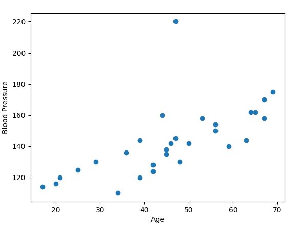
This fictional dataset shows the relation between the blood pressure of tested patients and their age.
The example above is a classic simple linear regression problem. We have one independent variable, which is the age, and one dependent variable, which is the blood pressure. Now we try to figure out a way to predict the blood pressure of the patient based on his or her age.
You can clearly see an upward trend, which could be described with a straight line:
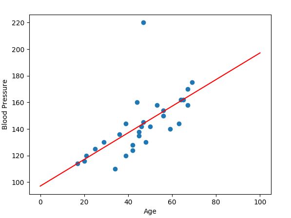
With the help of the line, we can clearly see that blood pressure increases with the age of the tested patients.
We can use this model (the line we drew through our data) to make a prediction (in this case, predicting the blood pressure based on the age).
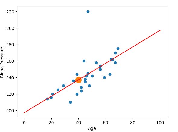
If you want to predict the blood pressure of a 40-year-old, say, you would take x = 40 and then figure out the corresponding value on the y-axis, which is approximately 137.
We are able to do this thanks to our best fit line (shown in red). This is the line that best represents our data. As you can see, using our best fit line we managed to make a prediction. But we only were able to make a prediction because we had the location of our best fit line.
The base equation for any line is y = mx + b, where:
- m is the slope
- x is the point we want to predict a y value for
- b is the y-intercept (the point where the line crosses the y-axis)
For the sake of simplicity, let’s look at an example with a very straightforward fictional dataset. This allows us to focus on our best fit line without being distracted by too many data points.
In the following example, you will learn how to draw a best fit line through a linear dataset and make a prediction using our constructed model!
Our dataset looks like this:
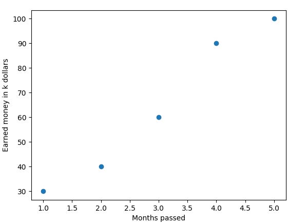
In this fictional dataset, you can see how much money a company has earned in x months. We’re using this simple dataset to start out with, but you can replace it with any other dataset that is worth modeling in a linear way.
I will be using Python, as it’s widespread and one of the go-to languages for machine learning. If you don’t know Python, you can either try following along anyway, as the code examples will be quite straightforward, or challenge yourself and implement the functions without the help of an external library in any other language of your choice (I explain how the functions work in the next section).
Before we get started, make sure you have sklearn, numpy and matplotlib installed. Open your command-line and type in these three commands:
pip install sklearn
pip install numpy
pip install matplotlib
We want to start in a blank Python file by making our imports:
from sklearn.linear_model import LinearRegression
import numpy as np
import matplotlib.pyplot as plt
The first import is our linear regression algorithm from sklearn. Sklearn is a machine learning library that implements common algorithms for easier usage. Then we import numpy, which is a widely used math library for Python. Finally, we import matplotlib for visualizing our dataset.
Next up, we define our features and labels:
X = np.array([1, 2, 3, 4, 5])
y = np.array([30, 40, 60, 90, 100])
The x values are the features. In this case, our features are the months that have passed. If you were to predict a type of animal, for example, your features might be its age, height, weight, etc.
The y values are the labels. In this case, the labels are the amounts of money the companies have earned. Think of them as the output you get. Again, if we were predicting animals, possible labels could be “Dog” or “Cat” (represented by 0 and 1).
We call np.array, as Python natively comes with lists only.
X = X.reshape(len(X), 1)
y = y.reshape(len(y), 1)
You don’t have to worry too much about this step in the beginning. Just know that we reshape the data into a form that the regression algorithm from sklearn can understand.
classifier = LinearRegression()
classifier.fit(X, y)
Now we initialize the classifier and call the “fit”-method for training our model, giving it our features and labels. In this case, training our model simply means finding the slope m and the y-intercept b.
m = classifier.coef_
b = classifier.intercept_
In order to draw the best fit line, we get the slope, which is a value between -1 and 1, and the y-intercept from the classifier, and store them inside of m and b.
plt.scatter(X, y)
plt.xlabel("Months passed")
plt.ylabel("Money earned in k dollars")
We now use matplotlib to draw our data points on the screen, and label the x-axis and the y-axis.
plt.plot([0, 10], [b, m*10+b], 'r')
Now we draw the best fit line our model just predicted, using the m and b we got out of the classifier. The first parameter we specify are the x-points. The first point goes from x = 0 to x = 10. Its y-coordinates are specified in the next parameter — y = b and y = m*10+b.
Therefore, the two points we connect to get our line are P(0, b) and Q(10, m*10+b).
The last parameter specifies the color ‘r’, which stands for red.
plt.show()
Finally, we display our finished plot.
This is how the code in its entirety looks like:
from sklearn.linear_model import LinearRegression
import numpy as np
import matplotlib.pyplot as plt

X = np.array([1, 2, 3, 4, 5])
y = np.array([30, 40, 60, 90, 100])

X = X.reshape(len(X), 1)
y = y.reshape(len(y), 1)

classifier = LinearRegression()
classifier.fit(X, y)

m = classifier.coef_
b = classifier.intercept_

plt.scatter(X, y)
plt.xlabel("Months passed")
plt.ylabel("Money earned in k dollars")
plt.plot([0, 10], [b, m*10+b], 'r')
plt.show()
If we run our program, we should see something like this:
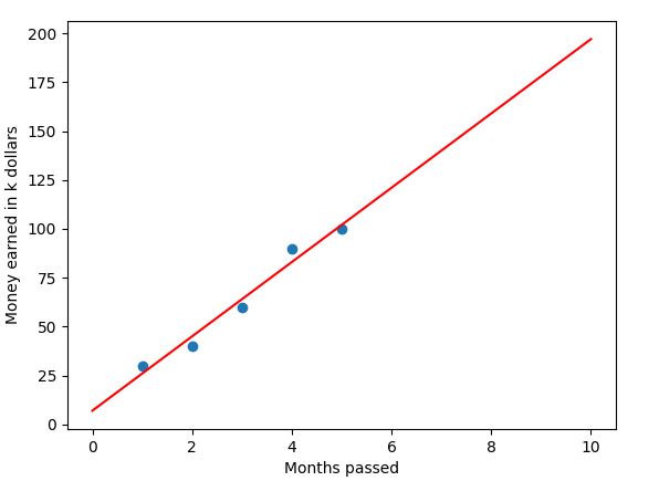
And voilà, you see our best fit line going through our data. It is important to mention that linear regression is obviously only useful when dealing with data with a linear relationship.
If you are working with a dataset which looks like this:
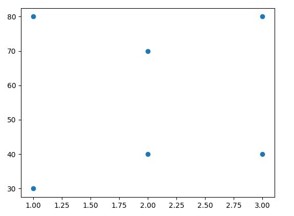
You will still be able to find a best fit line, but at the same time, that line will not be a good fit line, as it doesn’t represent your data very well.
How Regression Really Works
We have now successfully implemented a simple linear regression algorithm and drawn the best fit line on a fictional dataset using sklearn.
For the sake of understanding, let’s break down what happened behind the scenes:
As we have already said, our base equation for a line is y = mx + b.
These are the two formulas used to get m and b:
m =(mean(x) * mean(y) – mean(x*y)) / (mean(x)^2 – mean(x^2))
b = mean(y) – mean(x) * m
The mean refers to the average of a list, so basically, the mean of a list containing [-1, 1] would be 0.
To get the mean, let’s say for a list ‘x’, you have to get the sum of all elements and divide them by the length of the list:
mean_x = sum(x)/len(x)
When multiplying two numpy arrays, like in mean(x*y), you multiply each element of the list with its corresponding element of the other list, which has the same index.
Example: [3, 5] * [2, 4] = [6, 20]
Now that we have m and b, it’s easy to get the y-coordinate for any x we choose, by simply plotting them into our base formula.
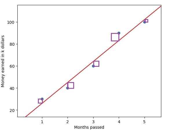
In this image, you can see the squared residuals of our best fit line (determined by the best fit line). A residual is the difference between the actual value of a point, and the estimated value.
A linear regression algorithm tries to minimize the sum of the squared residuals in order to find the best fit line, which resembles our dataset as closely as possible. The closer we manage to resemble our dataset, the better it will fit our data, and, therefore, our predictions will be more accurate. Have a look at this Image:
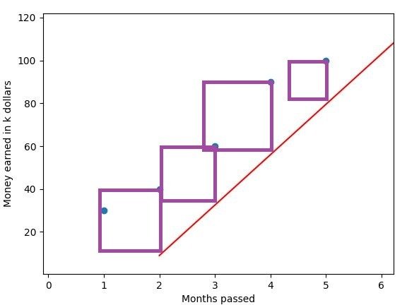
You see the same dataset with the squared residuals to a different line drawn in. Just by looking at it, you can see that the sum of residuals will be significantly higher than it was in the first plot, which indicates that this line is not the best fit line. A good way of finding out whether the line is the best fit line is to display it on the screen (using matplotlib, for example).
In this example, the closer we move the line to the left, the better our fit will be.
This is what we refer to as the Least Squares Method, because we try to find the best fit line by as much as possible minimizing the sum of the squares.
Using Machine Learning on the Web
All of these concepts can be used as tools by machine learning engineers, which is any Software Developer who knows and can use machine learning in their applications.
My recommendation would be to take a look at the Magenta Tensorflow Project to see what types of web applications people have come up with that involve Machine Learning.
I find this AI Duet Project especially interesting, which responds to your music input by continuing the sequence.
Other types of applications which make use of machine learning include stock predictors, which analyzes previous data to predict a future value, or Youtube, which uses machine learning to recommend videos to you based on what you have already watched.
We have barely skimmed the surface of machine learning. Simple linear regression is a very basic algorithm. Despite that fact, you can start using it straight away to make simple predictions. Other algorithms/concepts you might want to now investigate include K-Nearest-Neighbors, Support Vector Machines, Clustering, or the most hyped one, Deep Learning.
Pro Tip: Before looking at the links above, make sure to look up an ELI5 (Explain Like I’m 5) explanation of the terms, as it will give you a better, high-level overview of the concept, instead of overwhelming you with formulas at the beginning.
Expand Your Toolbelt

Thank you for reading this article. I hope it gave you a good introduction to and overview of machine learning!
Machine learning offers many possibilities, which are only limited by you. So, if you are interested in expanding your toolbelt as a backend developer, I suggest you to get your hands dirty with machine learning, thereby making yourself more versatile in the industry.
And although you most likely won’t be using it on a daily basis, it could give you an opportunity to work on some quite awesome projects in the future!
I would encourage you to play with it around and see if it is something that interests you.
Good luck on your path!
| Published on Web Code Geeks with permission by Gabriele Marcantonio, partner at our WCG program. See the original article here: Machine Learning for the Modern Web Developer Opinions expressed by Web Code Geeks contributors are their own. |